ANZ Finance blog | The Velocity of Money and CBDCs

The Velocity of Money and Central Bank Digital Currencies (CBDCs)

Published 8 March 2023

By Dr Peter J Phillips, Associate Professor (Finance & Banking) University of Southern Queensland

One of the most talked about issues in crypto-world is the idea of central bank digital currencies (CBDCs). CBDCs are digital currencies issued by a central bank. Like Bitcoin, but centralised.

I’m not one-hundred percent sure that central banks will be able to attract the talent required to launch and maintain their CBDCs but that is a discussion for another day. In this instalment, I want to link the idea of CBDCs with a classical idea from monetary theory: the velocity of money.

The velocity of money is the frequency at which one unit of currency is used to purchase domestically-produced goods and services during a period of time (usually a year). Put another way, it is the number of times each $1 “coin/note” changes hands within an economy each year or, perhaps even more simply, it is the rate at which people spend cash. The velocity of money is therefore a measure of the number of transactions between people within an economy.

We have talked previously about the connection between money supply and inflation. This connection is most clearly articulated by the quantity theory of money, which is encapsulated in a single equation:

MV = PQ

Here, M is the quantity of money in an economy, V is the velocity of money, P is the price level, and Q is the quantity of goods and services produced within the economy (i.e., output). PQ is nominal GDP (i.e., the total value of output at non-inflation-adjusted prices). The logical conclusion is that if V remains the same while M goes up, then unless output increases faster than the growth in money supply, prices (P) must also go up.

Extra goods soak up the extra money. If there’re no extra goods produced, the increase in the money supply just pushes prices up.

We can calculate V if we take PQ and divide by M. The data for nominal GDP, PQ, is readily available from the Reserve Bank of Australia (RBA). On the matter of money supply, we have a few choices. One of the most popular measures for M used in the calculation of money velocity is M1, which is the narrowest definition of money. It includes all the banknotes and coins plus liquid deposits such as savings account deposits. The data for M1 is also available from the RBA (see the RBA’s “statistical tables”). The total amount of M1 is reported each month, so I took the December value which in most years is the highest value for the year (i.e., money supply has grown during most years, though there might be a few down months here and there). The nominal GDP data are quarterly, so I summed them to give the GDP for the year. These measurements are summarised in Figure 1:

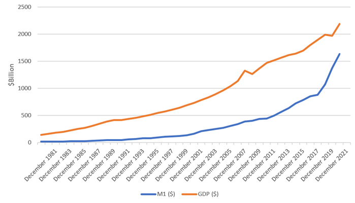
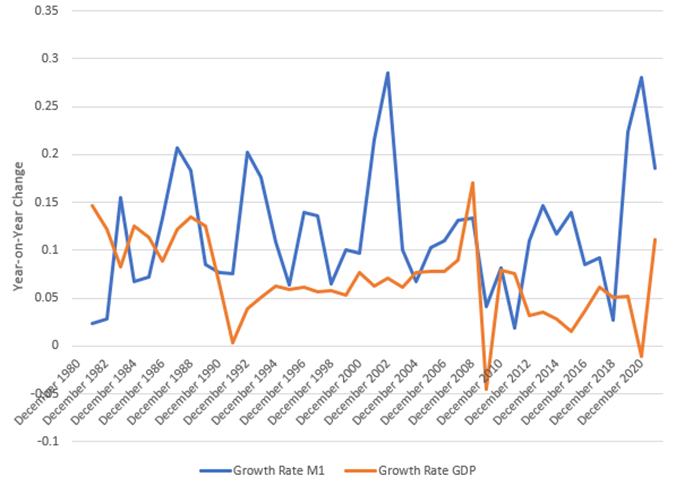
Notice how steeply the M1 supply has been increasing since 2017. In fact, for much of the time since 1980, the supply of M1 has been growing faster than nominal GDP. In Figure 2, I have plotted the growth rates (i.e., percentage change each year):

Figure 2: M1 and Nominal GDP, Annual Growth Rates

Now, you might ask, how come money supply has been increasing at such a rate and we haven’t had lots more inflation? The equation, MV = PQ, tells us that if velocity remains the same while money supply rises, there will be an increase in the price level unless output increases. Output has increased but that wasn’t the main reason why the consumer price level hasn’t reacted as much as one might have expected to the increase in money supply, until recently at least. The fact of the matter is that the velocity of money has fallen dramatically, meaning that the effect on the righthand side of the equation, PQ, of increases in M1, is diluted. Each additional dollar has been multiplied by an ever-lower velocity. Here is the chart of money velocity in Australia since 1980:

Figure 3: Money Velocity in Australia since 1980

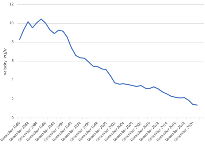
As you can see, the velocity of M1 money has fallen in Australia since 1980, from above 10 at one point to about 1.30. If velocity had remained at 10, say, then we would have had a much greater inflation problem if the quantity theory of money is correct. Instead of flowing directly into goods, the money is going somewhere else. In Australia, the most likely destination is real estate and the stock market. It is also likely that the increasing availability of “international investments” has played a role too.

A negative implication of low money velocity is that business is sluggish and central banks must work harder (print more) to get the stimulus they desire. At the end of the day, money velocity has been falling and that tends to dampen the effect of increases in the money supply on prices and output. What, though, you might ask, has this got to do with CBDCs?

Well, there’s a possibility, if CBDCs do get off the ground, that they might play some role in speeding up the velocity of money. One way that this might be accomplished is to make the digital currency unattractive as a store of value. That is, make people want to spend it rather than hold it. And make it unattractive to use for “bigger payments”. In the United Kingdom, the proposed Bank of England “Digital Pound” would have a holding limit of between 10,000 and 20,000 pounds. That means that digital pounds would have a higher velocity built in as a feature. While that might quicken the pace of business and foster more transactions within the economy, it might also push up prices.

Discussion Question

Do you think that CBDCs are a good idea? Will people embrace them? What do you think of the holding limit proposed in the UK?

Further Reading

For a discussion of the connection between the stock market prices and the velocity of money see:

Friedman, M. 1988. Money and the Stock Market. Journal of Political Economy, 96, 221-245.